Category: Supervised Machine Learning

One of the simples algorithms in Machine Learning is k-Neares Neighbors. It is considered a “lazy learning” algorithm where all the calculations are deferred until classification.
It works like this:
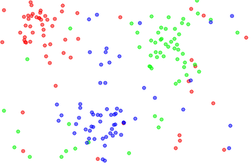
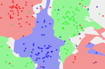
You have out training data with its features and labels. Then upon classification, or testing the data, you take the k-nearest neighbors and assign the label for your test feature with what the majority vote of the k-nearest neighbors is. If k=1 then your features label with be that of its closes neighbor.

The Dataset

The 1NN classification map

The 5NN classification map

(Images from: wikipedia)

When you have to deal with non-linear decision making, you can use decision trees to transform it into a linear decision surface.

Let say we have a buddy that goes wakeboarding if the weather is sunny but not windy. Whenever he sees the sun is up he considers going wakeboarding, but if it is too windy there will be too much waves on the lake and it is not as fun as when the surface is still. This data is not linearly separable, as shown in the following image: We can’t separate this with one line.

Decision trees enables you to make several linearly separable decisions one after another. In this case when we look at the data we can clearly see that it follows a pattern. First we can see that for instance if it is windy, he will not go wakeboarding regardless of if it is sunny or not. So by asking ourselves, is it windy? we can get a definite answer if it is windy, then we will not go wakeboarding.

If the answer was yes, we had an answer to our question if we shall go wakeboarding, and if it is not windy, we will ask another question: is it sunny? And if not, we won’t go wakeboarding, but if it is sunny, we’ll head to the lake.

This way, we could make a non linearly separable data set into a linear one by stepping through a decision tree.

 

If you then look at a little bit more complex data. You can see that for after a certain treshold on x, the data behaves differently. Here the data is not linearly separable.

This can be made into linear decisions using a decision tree.

Decision trees are easy to understand and interpret since they can be visualized as a tree structure. The data need not be prepared much whereas other methods may require normalisation. As we saw earlier that naive Base was good for classifying text, a decision tree is good when it comes to numerical and categorical data. They are, however, prone to overfitting. If some classes dominate in the training data, the generated tree may become biased. In that case the testing data needs to be balanced before training.

You want to find split points and variables that can separate the dataset into as pure subsets as possible, meaning that there the classes are preferably of only one type in the subset of the data. This is then done recursively with the generated subsets until you have classified the data.

Entropy (a measure of impurity) is what a decision tree uses to determine where to split the data when constructing the tree. Entropy is the opposite of purity, if all examples of a sample are of the same class, then the entropy is 0. If all examples are evenly split between all the available classes, then the entropy is 1.

Decision Trees use the entropy of a node to calculate what the split shall be.

 

P_i is a fraction of examples in the class i.

 

The way a decision tree affects its boundaries (choosing which features to make a split on) using entropy is by maximizing something called information gain.

Information gain = entropy(parent) – [weighted average]entropy(children)

 

See the example found in this video for an explanation about using information gain to choose which feature to use to split data in a decision tree.

 

 

Here you can find more information about decision trees: http://scikit-learn.org/stable/modules/tree

If you use the DecisionTreeClassifier in Scikit-learn you can tinker a bit with the parameters to set the criterions how it shall behave when splitting the train data into tree branches.

 

A Support Vector Machine is an algorithm that outputs a line separating two classes in a set of data.

An SVM will try to maximise the margin from the line to the nearest data points of the two classes.

If you use the scikit-learn library for training and predicting using the svm algorithm, you would use similar syntax as for the GaussianNB and in that matter the other machine learning algorithms.

In general when doing machine learning, you should reserve a part, about 10%, of your data to use as testing data, and that should not be used for training. Otherwise you would not get a realistic accuracy on your algorithm.

So we should split our training/testgin data into 4 varaibles, one set of features for training (an array, and in the case of svm, an array containing arrays that are the featuresw), one set of labels for those features, (the correct answer), similar variables to be used for testing.

from sklearn import svm
features_train = [[0, 0], [1, 1]]
labels_train = [0, 1]
clf = svm.SVC(kernel="linear")
clf.fit(features_train, labels_train)
pred = clf.predict([[2., 2.]])

 

If your data, however, is not separable linearly, lets say, that the data would look like this:

The data can not be separated by a line, but if you for instance add a new feature where the x is instead |x|, i.e. the absolute value of x, you could separate the data with a line.

A very powerful feature of support vector machines is to take a set of two dimensional data, and if it is not linearly separable, it uses something called Kernel tricks to transform the features into a multidimensional dataset, that is separable in order to get a solution

In the svm library you can also provide different kernels, or define your own. For instance, in the code example above you see that i use a linear kernel.

In the image below you see two decision boundaries that are produced on the same data but using two different kernels and another parameter called gamma, a linear to the left and rbf to the right (with gamma parameter of 1000).

The parameters are used when you create your svm classifier, ie. before you train it.

Another parameter you can use is called the C paramter. That can be set to indicate if you want a smooth border between the classes or classifier that classifies the training features correctly. The tradeoff can be that even though you could get a classfiier that is very correct on your training data with a high C, it might not be very good at generalizing your test data.

The gamma parameter tells how far a data point reaches in affecting the decision boundary. A low value means that you have a far reach, and a high value means a narrow reach. This means that with a high value you will get a very squiggly border, and a low value means you will get a more straight line because a single data point that otherwise would affect the border greatly, but might make the classifier not work well with the test data, is not affecting the line as much as it would be doing it only that dot would be the factor that adjusts the line. With a low value of the gamma parameter, you will also have the data points further away from the border to be taken into account when deciding where it shall be placed.

 

Overfitting

One thing we must always be aware of and try to avoid in machine learning is overftting. In the example below you see that the line to the left correctly classifies the green dots, but is very complicated. This can happen when you take the data too literal. If your algorithm produces a border similar to the one on the left instead of the one to the right, you are overfitting.

One way of reducing overfitting is through the use of you algorithms parameters.

Support Vector Machines work very well in complicated domains where there is a clear margin of separation. They do not perform efficiently in very large data sets, the training time increases cubically. They also do not work very well where there is a lot of noice in the data where the classes overlap (in that case a Naive Bayes classifier would be better)

Naive Bayes Classifier is a probabilistic classifier used in supervised machine learning that is especially useful when categorizing texts. They apply Bayes’ Theorem which describes the probability of an event to take place based on given knowledge of conditions related to the event.

Where A and B are events and A != B
P(A) and P(B) are probabilities of observing A and B without regards to each other.
P(A|B), a conditional probability of observing A given that B is true.
P(B|A) is the probability of observing B if A is true.

One example of a library where you can use a Gaussian Naive Bayes classifer can be found in the scikit-learn python library sklearn.naive_bayes.GaussianNB with which you can train (fit) to tell wether a feature match a label.